Smooth Signals by Filter or Moving Average
When monitoring and controlling signals, we frequently have AIs (analog inputs) with noise and/or oscillations. “Noise” in this context is a meaningless or irrelevant fast variance in a signal. These can be caused by the measurement technique, the nature of the process, electrical interference, badly tuned PID loops, or other factors. When fed to logic such as PID loops or pacing references, these noisy inputs can cause undesirable oscillations on outputs to motor speeds, valve positions and other AOs (analog outputs) while generating operator confusion.
As with all engineering, we must balance the trade-offs – in this case between the competing demands of responsiveness vs smooth stability. Too responsive and we can prematurely wear out components & cause upsets to nearby processes. Too smooth and we can spend long periods of time out of optimal control. In general, the more smoothing (the longer the time constant), the less integral action any PID loop using that signal as a PV (process variable) can tolerate without generating its own oscillation.
Smoothing Filters
Filters, the short version:
The longer the time constant, the smoother the result.
Filters, the long version:
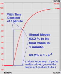
An exponential filter asymptotically moves an output toward its input by the same % every time period. So the output moves faster toward the input the farther away it is, slowing as it gets closer. This trend shows what happens when the input to a filter with a 1-minute time constant changes from 0 to 100. You can see it approaches fast at first, then slows, and never quite gets there. Because of stuff I learned decades ago in difficult differential equations & then mostly forgot, the signal moves 63.2% (1-e-1) from the initial to the final input in its time constant. We say “it never quite gets there” in an idealized situation like the one pictured here. But on a real-life noisy signal (the whole reason we are having this conversation), it really does “get there” when a noisy signal makes a significant change – the smoothed signal will intersect the noise range of the input within a few time constants.
If you’re working in a modern PLC or DCS, there is likely a filter block available to you – you just connect it between your AI and PID blocks, set the time constant, and you’re done.
Coding a Custom Filter
However, if your PLC does not have a filter function, it’s easy to code one.
The simplest method is to consider the fundamental concept of a filter – it adds most of the previous output to a small portion of the input each scan. So you can compute:
OUT = ( OUT × (1 – F)) + ( IN × F )
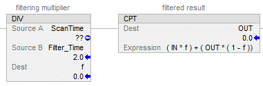
where F is a smoothing factor. 0.2 would be a little bit of smoothing, and 0.001 would be very smooth. F=0 would just never change the OUT. F=1 would not smooth at all – it would just set OUT to IN each scan.
An optional step is to calculate F based on a desired time constant. To do this, divide the time since the block last scanned by the desired time constant. So if you have a PLC task scanning at 20 ms and you want a 5 second time constant, your F will be = 0.020÷5.0=0.004. The PLC will add 0.4% of the input to 99.6% of the previous output every scan, and that gives you an exponential filter. Also note if the time constant is shorter than the scan rate, you’ll end up with F>1, which is undesirable. You should code to trap that condition and just set OUT=IN instead of performing the filter calculation.
Avoid the NaN Filter Pitfall!
Without coding protection, if a bad value (NaN = “Not a Number”) is passed to the filter input, the output will also become NaN and will get trapped so that even after the input goes good again, the filter will stay NaN without manually setting the OUT to a valid number. Sources of NaNs include division by zero, fraction powers (like square roots) of negative numbers, or inputs that report NaN on bad quality. The method of detecting and rejecting NaNs varies according to the PLC. With the AB Studio5000 family processors, You can have OK =(( X < 120 ) and ( X > -120 )), and act accordingly if it’s not OK.
Moving Averages
Filters are good for smoothing generally noisy signals. However, if a signal has noise that oscillates with a repeatable period, a better method is the MAVE (Moving Average). Unlike a filter which only needs an input, and output, and a time constant, a MAVE requires a timer to trigger it, and a sample buffer. You’d want at least 10 samples, with 20-60 being typical.
When triggered, a MAVE collects a REAL (floating point) sample to overwrite the oldest sample, then sets its output to the average of all the samples. Some have an option to adjust weights, but that is not desirable for this application.
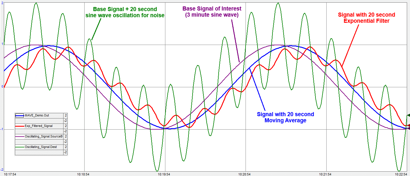
First let’s consider the idealized way a MAVE can remove short-term oscillations from a signal to reveal only the significant signal underneath that oscillation. The oscillating signal in this trend is a 20-second sine wave (green) added to a 3-minute sine wave (purple). We want to eliminate the 20 second noise and only look at the 3 minute wave. The MAVE (blue) has a 20 sample buffer and samples once per second. Its output almost perfectly matches the base signal of interest with the influence of the noise completely removed. The down-side is the output of the MAVE represents what happened 10 seconds ago, not what is happening now. By contrast, while a 20-second exponential filter (red) dampens the noise, it does not remove it.
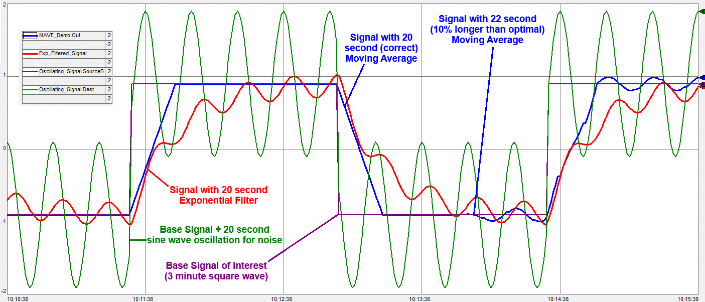
Another idealized scenario to show how MAVEs and filters work – this time instead of a 3 minute sine wave, the base signal we are interested in is a 3-minute square wave. As expected the MAVE takes 20 seconds to go from the old value to the new value – but it fully matches the new value in 20 seconds, and as before completely removes the noise. By contrast the filter does not remove the noise, and takes about a minute for its oscillation to include the base value.
This trend also shows the difference between a perfectly tuned MAVE with a period exactly matching the oscillating noise (the first 3:20, versus a MAVE with a period deviating 10% from the period of the oscillation (the last 1:40). You can see the MAVE still helps smooth the signal, but no longer completely removes the noise. So we are using a MAVE as a notch filter – passing on the signal without oscillations at a specific frequency.
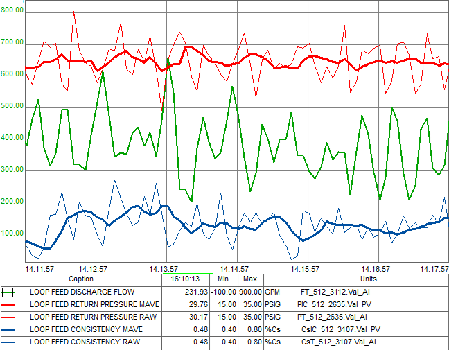
How do MAVEs perform in real life? The trend below shows a signal (loop feed discharge flow) that wildly oscillates due to the actions of equipment outside the system’s control. That causes significant effects on four other signals I do control. Shown in this trend are two of those signals – return pressure and consistency. The raw oscillating signal is shown as the thin line, and the output of the MAVE is the thick line. I zoomed in on the scale so you can see the MAVE signal is still moving around, but the effect of the oscillating signal is removed from its variability so that I’m left with a signal good for control.
With a 20 sample buffer, you would have a timer that triggers a MAVE sample every 1/20 of the oscillation period. If the system itself is doing something periodically to cause oscillations, you can just divide that timer preset by 20 to get your sample trigger timer present. Example – solid fuel furnaces sometimes feature grate shakers that run 2-3 seconds out of every minute. When they shake they upset signals around the furnace (particularly O2). Running those signals through a MAVE that averages samples for exactly one shake period will remove the effect of the shaker from the signal and allow you to monitor and control the other effects such as fuel/air ratio, etc.
Note – do not reset your sample timer when it is done – that takes at least one scan to reset, and may spend another scan at zero time when it should be counting up. In an AB PLC if you’re using a TON, set its PREset to a large number (like a billion milliseconds). When its ACCumulator exceeds your sample trigger preset, trigger the sample and subtract the sample preset from the ACC and let the timer just keep running. Two pitfalls to avoid here:
- Make sure your timer DN bit never gets set. If it does, it will stop timing. I usually reset the timer and set its preset to 1000000000 in a first scan routine to avoid that.
- Never set the ACC or PRE to a negative number. That will major-fault the processor.
Auto-Adjusting MAVE Period
In the above example the oscillation is caused by a collection of 20 pieces of equipment that periodically open and close their valves. The periods vary somewhat… when they are mostly synchronized, the oscillation we see is particularly large. Since the period is variable, I wrote code to set the MAVE period to the observed noise period. It does so by:
- Capture the range – the recent min and max signal. To do this, Range_Max continually drops by a small decay amount (0.5 GPM / second) but rises to the actual signal if it is higher. Likewise Range_Min rises by a small decay amount but falls to the actual signal if it is lower.
- Range_Span = Range_Max – Range_Min
- Range_Rising_Trigger = Range_Min + Range_Span × 0.6
- Range_Falling_Trigger = Range_Min + Range_Span × 0.4
- Continuously run a timer.
- When the signal falls below Range_Falling_Trigger, turn the period capture bit off.
- When the signal rises above Range_Rising_Trigger with the period capture bit off, turn it on – this is a one-shot condition indicating the start of a new noise oscillation period.
When that one-shot occurs, we ensure the elapsed time is reasonable (in this case between 15-40 seconds), and Range_Span ≥ 100 GPM. If any of those conditions aren’t met – that’s fine, we just reset the timer anyway but do not update the period because the oscillation period of the signal was not clear.. But if all those conditions are all met, we:
- Capture the elapsed time before resetting it – that is the duration of the most recent period.
- Filter that into the smoothed period (0.9×Smoothed_Period + 0.1×Recent_Period).
- Divide Smoothed_Period ÷ Number_Samples to set the MAVE trigger timer.
The result is a MAVE which accurately averages samples across exactly one oscillation. The Process Solutions Group at Cross Company has experience imlementing solutions like this to improve process operations. We aim to help customers improve quality, raise efficiency, and lower risk in their operations. Reach out and start a conversation with one of our experts today!